Introduction

Industry has numerous articles about PID (proportional, integral, derivative) controller loop tuning and its various approaches. From complex mathematical algorithms to various tuning techniques, loop tuning often presents itself as a black box that requires a certain mathematical artistry to open. One way to open this box is to ask:

“What kind of process is being controlled?”

Accumulating vs Non-accumulating processes

Most processes can be categorized as either accumulating or non-accumulating. By accumulating, we mean that the process is collecting or holding material or energy, such as levels and some temperatures and pressures. A non-accumulating process would be flows, where a change in the control device almost instantly translates to a change in the process measurement as well as hydraulic pressures.

• Accumulating – Processes where material or energy are accumulated or held. Levels are accumulating because they hold volume or mass. Vapor pressures can be accumulating as they accumulate gas. Some temperatures are accumulating because they hold heat capacity.
• Non-accumulating – Flows, hydraulic pressures, and temperature due to combustion.

Basis for integral time

Why is identifying if the process is accumulating or non-accumulating important? Integral time is based on the time it takes a process to accumulate (see figure 1). For example, if it takes about 5 minutes to fill a tank halfway at full feed, the integral time will be about 5 minutes. Conversely, the time it takes for a change in valve position to reach the flowmeter is a matter of seconds. This would be a good start for the integral time for the flow.

This general rule is at play. The integral time (in time per repeat) is relative to the accumulation time. A large time to accumulate means a large integral time; conversely, a short accumulation time means a small integral time.

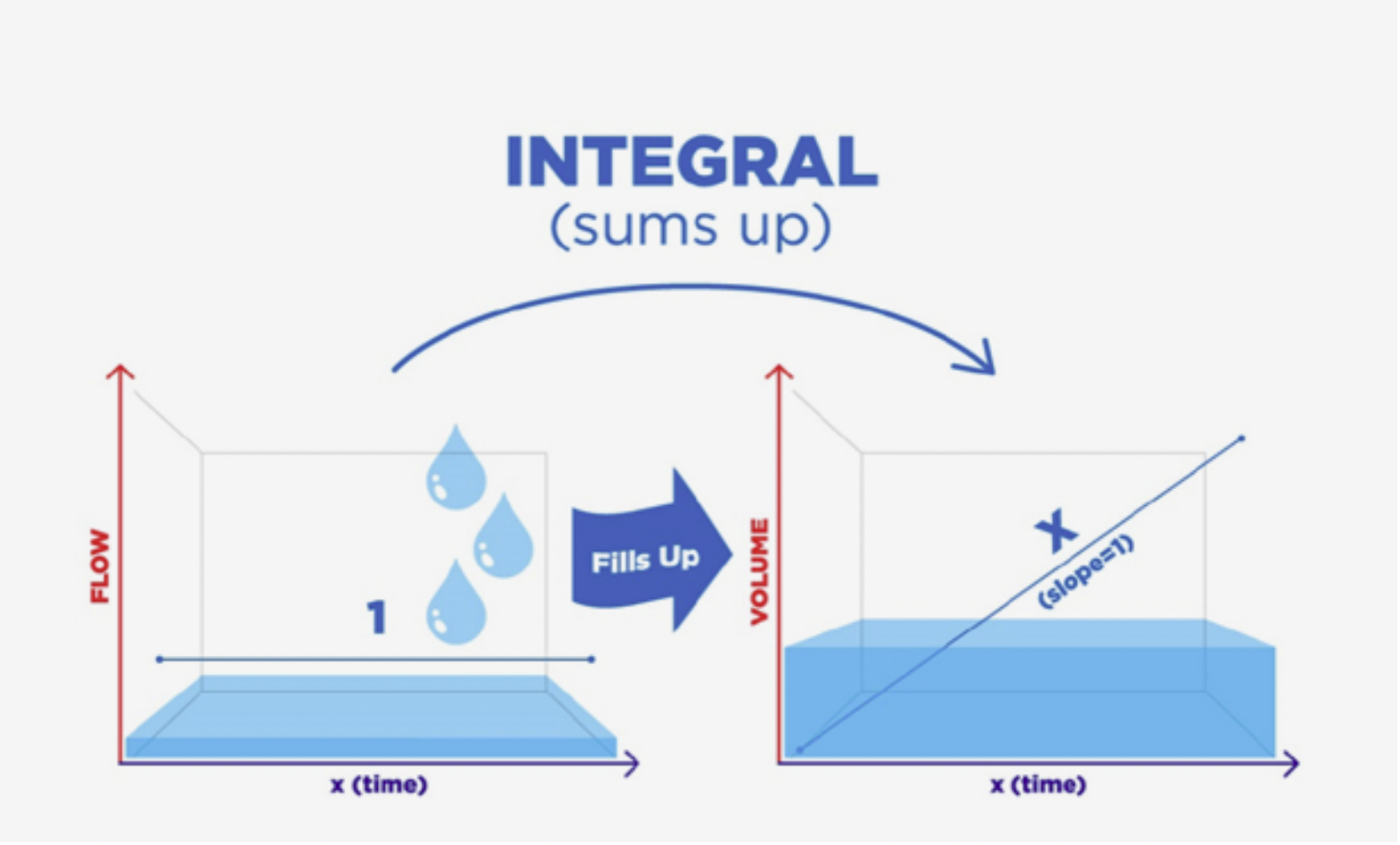
Why it's called integral

Integral is essentially a process where the material or energy ‘sum up’, accumulate or in mathematical terms, integrate. This knowledge is key to understanding how to tune various processes AND why classifying them as accumulating or non-accumulating makes a difference.

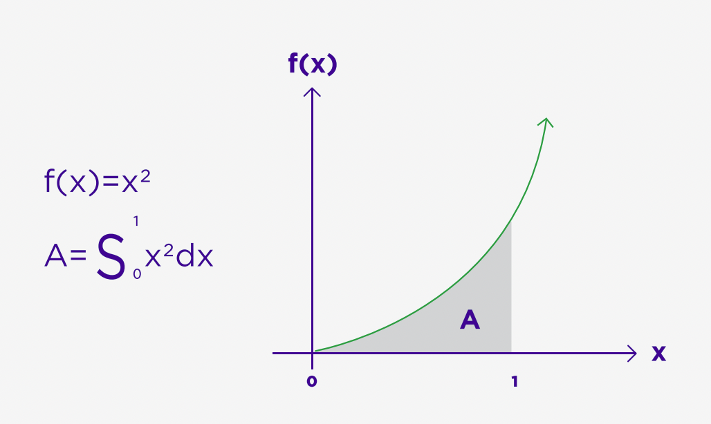
Accumulation can then be thought of in the mathematical integration term where we calculate the area under a curve (figure 2). In this view, the area is relative to the mass accumulated, and the integral time is relative to the accumulation time.

Figuring the integral

Let’s take a closer look at an accumulating process to begin figuring the tuning. We’ll start with integral time based on the discussion above and our understanding of how integral time relates to process accumulation.

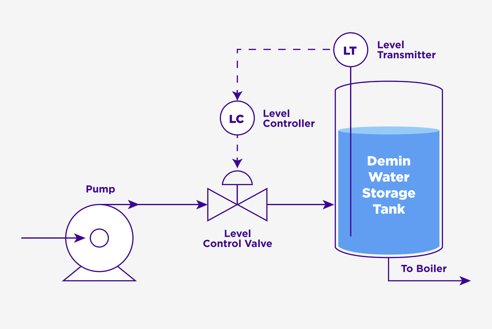
Let’s say a tank (figure 3) holds 10,000 gallons of demineralized water and that the maximum feed rate is 1,000 gallons per minute. It’s not hard to determine it would take 5 minutes for the tank to fill halfway. Obviously, the larger the vessel and/or the smaller the feed rate increases the time to accumulate the level.

Piecing all this together tells us that since the accumulation time for a level tends to be long, then the integral time should also be long. Thus, the time it takes to fill or empty a level is relative to the integral period. Assuming we are using minutes per reset, we might look at 5 minutes for a starting point for the integral time of our tank. Later we can fine tune by introducing upsets (setpoint bumps) to get the desired recovery we want.

Figuring the proportional

Now let’s look at the proportional term. Clearly, if the tank fills or drains suddenly, we want the controller to react even to the point of moving the output to its limits. If we imagine the proportional term like a seesaw where the fulcrum moves changing the proportion of the weight needed on each end to balance, we can start to determine the kind of proportional gain required.

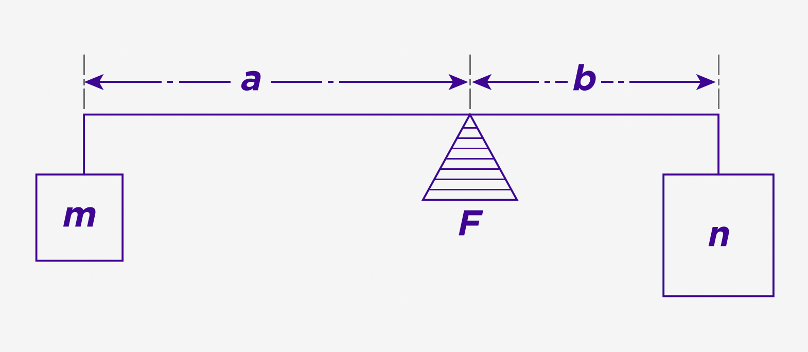
In figure 4, “m” represents the desired output to the control valve while “n” represents the error from the desired setpoint. The ratio “a/b” would then represent the proportional gain. Using some real numbers, let’s say the desired setpoint is 50% level. Let’s say the measurement is 25% creating an error of 25%. Now, we want our control valve to be at maximum output at that point. The gain then becomes 100/25 or 4. Another way to look at this is again by looking at the size of the tank. Let’s say it’s a 10,000 gallon tank passing 1,000 gallons per minute max. Now we have another proportion of 10 to 1. So depending on how tight we want the control and how large the vessel is the gain could be anywhere between 4 and 10!

In most cases when looking at a level, the proportional gain should be 1 or greater. In that way, we move the output at least at a 1-to-1 proportion to the error so that the valve is at the extremes when the vessel is near full or near empty. Imagine that normally the controller sits with the valve halfway open, and we are trying to maintain the level at half full or 50%. To get the valve fully opened or fully closed when the tank goes empty or full means putting the proportional gain at least at 1. In other words, we want full travel of the valve over the range of the level using proportion.

Typical proportional integral relationship

So now we’ve created a rule of thumb for P & I terms regarding our level. P (proportional gain) needs to be greater than 1, in this case we decided on a range of from 4 – 10. I (integral time) needs to be long, in minutes not seconds. In this case, we decide on 5 minutes based on fill time. Note there are ALWAYS exceptions to any rule, but this gives us a decent starting point. Notice that the Proportional is large (fast) and the Integral time is long (slow). This relationship tends to hold true for all processes, that is that conversely a process that requires a short (fast) integral time also has a small (slow) proportional.

Non-accumulating processes

Now let’s look at a non-accumulation process, such as flow, so we can see the difference in tuning and if this fast-slow relationship holds. When we change the output to the control valve, we get an immediate change in the process variable (flow). So, there is little accumulation. Where it takes a lot of time to accumulate materials in a level, it takes almost no time for the process to react in a flow.

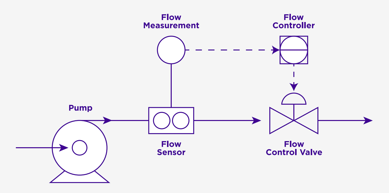
In figure 5, we can determine the time it takes for the material to flow down the line from the sensor to the control valve. In most cases, we are talking a matter of a few seconds. From this determination, we can conclude the integral time is fast, let’s say 5 seconds.

Now let’s look at proportional action. For a level, it took a large change in valve position to make a small change in the level. For a flow, we see that a large change would immediately move the flow rate to an extreme. So, we know we want a smaller ratio (think back to our seesaw), almost certainly numbers less than 1.

Key tuning questions

Now, the questions we really need to ask in order to tune our process are:

• How large is it?

  Size - its largeness gives us an idea where our proportional term stands.

• How long does it take?

  Time – the period it takes to move from one value to another gives us an idea where our integral time should be.

Keeping size and time in mind, we can take a quick look at other types of process conditions and controls.

Hydraulic Pressure – Hydraulic pressure acts much like a flow. As soon as we adjust the control output, we see a rapid change in pressure. So, like most flows we would expect short integral times and small proportional gains. Example: P=0.5; I=20s.

Vapor Pressure – Since gas is compressible, it has an accumulating behavior. This is especially true when we are talking about head pressures in a vessel. We can expect larger proportional terms and longer integral times. Example: P=2; I=120s.

Temperatures – This is where most people struggle as it’s hard to figure out how long it takes to get a BTU through a brick. Actually, BTUs and where they are going is key here. If we are generating BTUs in combustion, we can see changes rapidly, whereas if we are transferring heat it takes time. By considering the heat capacity – the time it takes to generate and move the BTUs – we can get some idea of what the tuning might look like.

For example, a tray temperature in a distillation column would take significant time to get there, but once it got there, it might change quickly. Making a step change in the control output can give us an idea of what the time period is and help us pick an integral time. The amplitude ratio between the change in output and the change in temperature can give us some idea on proportional gain.

Again, we just want to know the size (proportion of output to process change) and how long it takes (integral time).

Derivative / Rate of change

Derivative action – also known as rate of change – should be rarely used. Its best use is for “excursion control.” This is when a process has some force within it that causes a rapid change. For example, the kickoff of many reactions will cause a sudden temperature rise followed by a rapid fall in temperature. Figure 6 illustrates such an excursion.

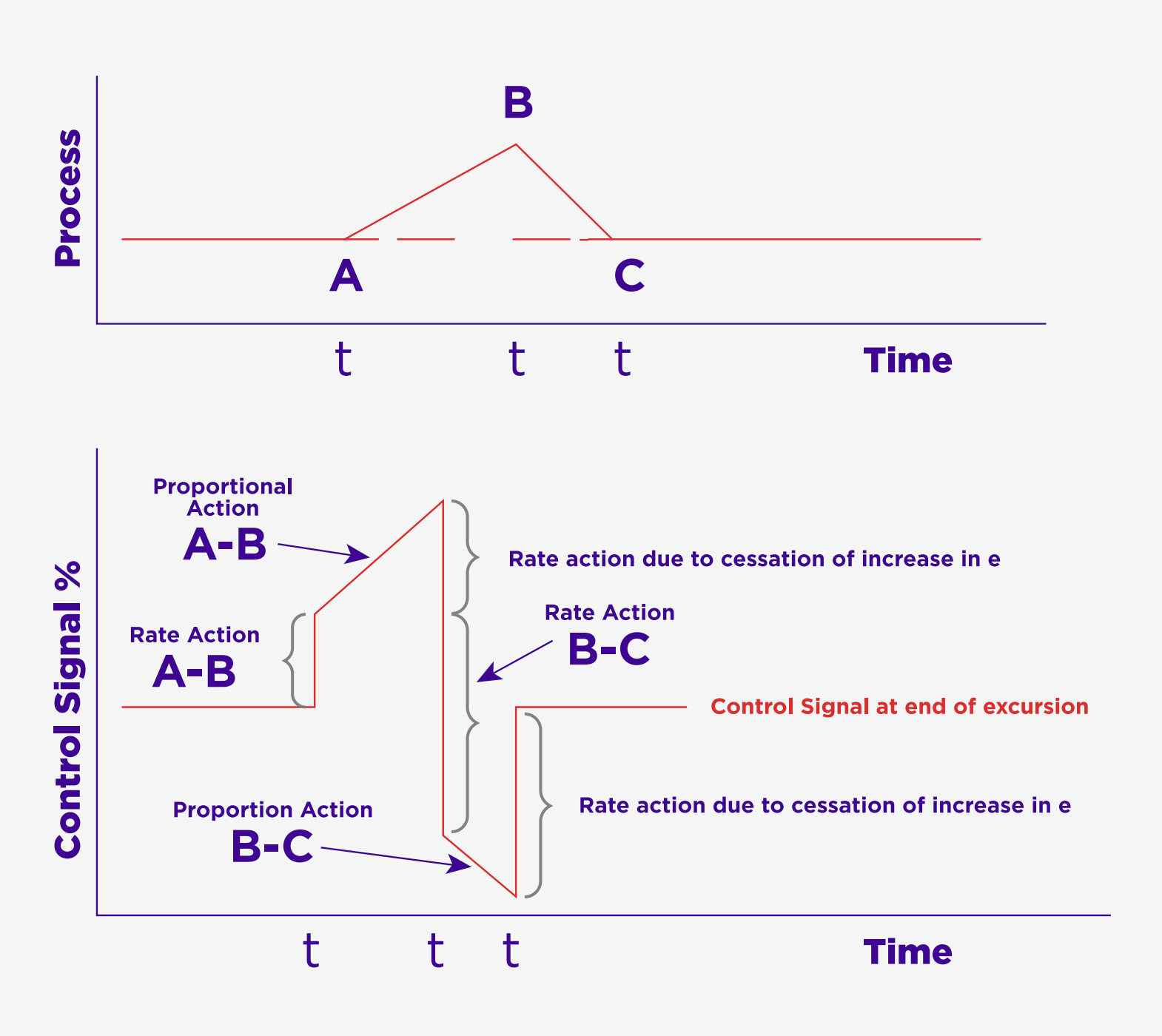
While integration is about accumulation and finding the area under a curve, derivative can be looked at as the rate of change or the slope of a curve.

Fine tuning

In summary, proportional is all about size, integral is about how long it takes, and derivative is about sudden change. Understanding the basic behavior of your process can go a long way to deciding where to start tuning-wise. After that, we perform some fine tuning by making changes to the setpoint and some adjustments to get the kind of curve preferred, most typically quarter wave decay where each successive swing is 25% of the previous.